
Multilayer Planning with the WAN Automation Engine
Overview
The WAE network model includes the multivendor devices that participate in the IGP (OSPF or IS-IS) and can be extended to include the DWDM topology. Using the WAE Design application or WAE APIs, you can use the model to simulate “what if” scenarios and optimize paths for L3 and L1 domains. The purpose of this tutorial is to demonstrate the multilayer capabilities of WAE.
Note:
- The network model used in this tutorial is from the WAE Design samples directory: us_wan_L1.txt
- If you don’t have the WAE Design application, see the tutorial Using dCloud to Access the WAN Automation Engine Demos.
- If using dCloud, use the US East datacenter and launch the demo for “WAE Live”. The WAE Design application will be on the workstation desktop.
Discovery of the DWDM Topology
The goal in multilayer discovery is to augment the WAE model of the IGP with the DWDM topology. For Cisco optical, the layer 1 topology discovery and mapping between the L1 circuit path and the L3 adjacency is automatic; WAE can interface through CTC to the NCS 2K running 10.6.2 or later to discover the DWDM topology and L3-L1 mapping if LMP is configured on both the NCS 2K and IOS-XR. In IOS-XR, an example of the LMP configuration is shown below:
RP/0/RP0/CPU0:Napoli-5#show run lmp
Mon Aug 21 19:31:21.657 CET
lmp
gmpls optical-uni
  ...
  controller dwdm0/6/0/20/0
   neighbor Battipaglia
   neighbor link-id ipv4 unicast 20.20.20.60
   neighbor interface-id unnumbered 2130707466
   link-id ipv4 unicast 20.20.20.50
  !
  ...
  neighbor Battipaglia
   ipcc routed
   router-id ipv4 unicast 10.58.244.11
  !
  router-id ipv4 unicast 10.58.244.50
!
!

RP/0/RP0/CPU0:Napoli-5#show run int hundredGigE 0/6/0/20/0
Mon Aug 21 19:31:38.179 CET
interface HundredGigE0/6/0/20/0
  description Core Link to Salerno - bundle member
  bundle id 2 mode active
  cdp
  transceiver permit pid all
!

RP/0/RP0/CPU0:Napoli-5#show run controller dwdm 0/6/0/20/0
Mon Aug 21 19:31:59.844 CET
controller dwdm0/6/0/20/0
  g709 enable
  g709 fec high-gain-sd-fec
  wavelength 50GHz-Grid frequency 19315
  admin-state in-service
!
For third party optical vendors, typically WAE will use the vendor specific NMS for the topology details and populate a vendor agnostic YANG model. Third-party interfaces for L1 vendors require a WAE function pack. Please contact your Cisco sales representative for details.
Multilayer Planning in WAE Design
WAE Design has visualization, simulation and optimization tools and capabilities for multilayer planning scenarios. This section will cover a few of these scenarios by example. You can follow the examples using the us_wan_L1.txt plan file located in the WAE Design samples directory.
Example: Visualize the Multilayer Topology
- Open us_wan_L1.txt and make sure you have the network plot set to the Simulated Traffic view.
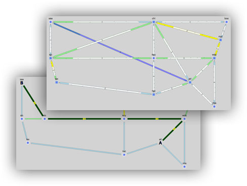
- Currently you are looking at the layer 3 topology. View the layer 1 topology by selecting the L3/L1 toggle button in the upper left corner of the Design application.
- From the layouts menu, select the layout “Joint” to see a layout that was setup to see the L3 and L1 views in the same plot.
- See the settings for this layout by right clicking an empty area of the plot and selecting Plot Options. Then toggle to the Layer 1 tab to see available options.
- In this plot, you can also open any site to see the contained L1 and L3 nodes.
Another useful tip is the ability to select background objects in the network plot. To enable this setting, go to View -> Preferences and check the box that says “Enable Selection of Background Objects”. 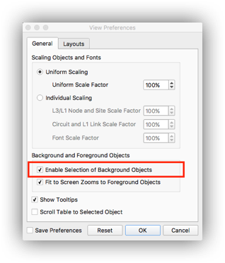
Example: Simulate the Impact of a Fiber Cut
The primary purpose of WAE including the layer 1 information is to understand the impact to the layer 3 topology.
- Using us_wan_L1.txt ensure you have the network plot set to the Simulated Traffic view.
- Highlight a layer 3 circuit, toggle to the L1 view and observe the associated layer 1 circuit
- Click an empty area of the plot remove the highlights for the selections
- Right-click a layer 1 link and select Fail
- Observe the impact of the failure in the L1 and L3 views
- Right-click and empty area of the plot and select Recover and select the L1 link.
Example: Modeling DWDM Circuit Paths and Protection Schemes
In the previous example, failing a L1 link simulated the impact to the layer 3 topology. In WAE, layer 3 circuits are mapped to layer 1 circuits, and layer 1 circuits can have circuit paths. In this example, you will use circuit paths to simulate optical restoration and 1+1 protection scenarios.
In WAE, L1 links have properties for distance, delay, loss, metric, feasibility metric, reserved L1 circuit paths, maximum L1 circuit paths and waypoint information. This information helps determine the path of the L1 circuit (which can have a feasibility limit). The colors on the L1 links represent the utilization, which is the number of active and operational circuit paths routed through the L1 link divided by the maximum allowable.
Simulate Optical Restoration
- Using us_wan_L1.txt ensure you have the network plot set to the Simulated Traffic view.
- In the L1 view, right-click on the L1 link between SLC and KCY and select Filter to L1 Circuits Through L1 Links.
- In the L1 Circuits table, identify and select the L1 circuit between CHI and SEA
- Right-click an empty area of the plot and select New -> Layer 1 -> L1 Circuit Paths
- For the 1 selected L1 circuit, set the path option to 2 Uncheck the Standby box.
- In the L1 Circuits table, identify and select the L1 circuit between CHI and SEA then right-click on the L1 link between SLC and KCY and select Fail
- Observe the dashed line for this circuit. This failure simulation shows path option 1 becoming non-operational and path option 2 becoming operational.
- Right-click and empty area of the plot and select Recover and select the L1 link.
Simulate 1+1 Protection
- Using us_wan_L1.txt ensure you have the network plot set to the Simulated Traffic view.
- In the L1 view, right-click on the L1 link between SLC and KCY and select Filter to L1 Circuits Through L1 Links.
- In the L1 Circuits table, identify and select the L1 circuit between CHI and SEA
- Right-click the circuit and select Filter to L1 Circuit Paths.
- Open the Properties menu for the L1 circuit path with path option 2. (This was added in the previous example)
- Set the checkbox for Standby and ensure the checkbox for Active is also checked.
- To modify the path, select Insert After and set site SLC to Exclude.
- Select OK to exit the properties menu
- In the L1 Circuits table, identify and select the L1 circuit between CHI and SEA then right-click on the L1 link between SLC and KCY and select Fail
- Observe the circuit path change for this circuit. This failure simulation shows path option 1 becoming non-operational and path option 2, which was already established becoming operational.
- Right-click and empty area of the plot and select Recover and select the L1 link.
In this example, you changed the L1 circuit path manually to be partially disjoint from the other. In WAE Design version 7, there is an optimization tool to compute disjoint L1 circuit paths.
Example: Multilayer Optimizations for Segment Routing Policies
If the layer 3 and layer 1 topologies are included in the model, you can take advantage of the WAE optimization tools for Segment Routing Policies.
Optimize a SR Policy for Latency and Avoidance
This example will use the WAE SR-TE optimization tool.
- Right-click an empty area of the plot and select New -> LSPs -> LSP
- In the LSP Properties menu, set the type to SR, set the source to er1.sea and set the destination to be er1.atl. Click OK.
- Observe the path of the SR policy.
- Next optimize the SR policy by selecting Tools -> SR-TE Optimization
- In the SR-TE Optimization menu, set Minimize Path Metric to Delay and ensure Avoid Nodes is set to None. Click OK.
- Observe the optimized path of the SR policy in the new plan file.
- If you want the lowest latency SR policy that avoids nodes in site KCY, first highlight the site KCY, right-click and select Filter to Contained Nodes.
- In the Nodes table, highlight the selected nodes.
- Select Tools -> SR-TE Optimization. In the SR-TE Optimization menu, set Minimize Path Metric to Delay and set Avoid Nodes to “Selected in Table”. Click OK.
- Observe the optimized path of the SR policy in the new plan file.
In this example, the avoidance criteria is referring to L3 nodes. In WAE Design version 7, you can also select avoidance criteria for L1 Nodes and L1 Links.
Optimize SR Policies for Multilayer Disjointness
In this example, you will use WAE to compute paths for SR policies that are disjoint for the L3 and L1 topologies.
- Close any open plan files and do not save changes. Open the plan file us_wan_L1.txt. It should be in the original state in which you started this tutorial.
- Right-click an empty area of the plot and select New -> LSPs -> LSP
- In the LSP Properties menu, set the following parameters:
- Type: SR
- Source: er1.sjc
- Destination: er1.kcy.
- In the Advanced tab set Disjoint Group to any string such as ‘group1’.
- Click OK.
- Right-click on the LSP in the LSPs table and select Duplicate
- Select the LSPs in the LSPs table, right-click an empty area of the plot and select New -> LSPs -> LSP Paths. Leave the defaults and click OK.
- Select Tools -> LSP Disjoint Path Optimization.
- In the LSP Disjoint Path Optimization menu, set the following options:
- Disjoint Routing Selection: Create Disjoint Paths between LSPs in Disjoint Groups.
- Priorities: set L1 Links to 1
- Click OK.
- Observe in the new plan file that the SR policies are disjoint at L3 and L1.
Example: Capacity Planning Optimization
WAE has a tool called Capacity Planning Optimization that attempts to get below a simulated utilization threshold by upgrading the capacity in some way. This section will show some of the options of the tool and the results.
Before you start this section, do the following tasks.
- Close any open plan files and do not save changes. Open the plan file us_wan_L1.txt. It should be in the original state in which you started this tutorial.
- Right-click an empty area of the plot and select New -> Demands -> Demand
- In the Demand Properties menu set the following options:
- Name: Can be any string such as ‘new_customer’
- Source: er1.sea
- Destination: er1.atl
- Traffic: 700 (Mbps)
Capacity Planning Optimization Create Parallel Circuits
- Select Tools -> Capacity Planning Optimization
- In the Capacity Planning Optimization menu, select the following options:
- Maximum Interface Utilization: 80
- Capacity Increment: 1000
- Upgrade Existing Circuits: Create Parallel Circuits
- Create New Adjacencies: Restrict New Adjacencies between Nodes None
- Select OK
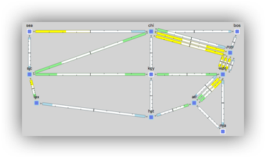
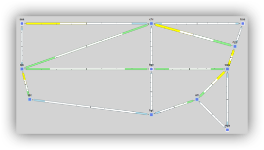
The result should look similar to the picture on the right.
Capacity Planning Optimization New Adjacencies (with Optical Bypass)
 Ensure the plan file us_wan_L1.txt is selected. This example will examine a case where you can only add new adjacencies between core nodes. First, select only the core nodes in the Nodes table.
- Select Tools -> Capacity Planning Optimization
- In the Capacity Planning Optimization menu, select the following options:
- Maximum Interface Utilization: 80
- Capacity Increment: 1000
- Upgrade Existing Circuits: (Ignore)
- Create New Adjacencies: Restrict New Adjacencies between Nodes Selected in Table (22/33)
- In the Layer 1 tab, select the checkbox Create L1 Circuits
- Select OK
The result should look similar to the picture on the right.
Capacity Planning Optimization LAG Augmentation
 Ensure the plan file us_wan_L1.txt is selected This time you will see what happens if you can only augment existing LAG members.
- Select Tools -> Capacity Planning Optimization
- In the Capacity Planning Optimization menu, select the following options:
- Maximum Interface Utilization: 80
- Capacity Increment: 1000
- Check the box Use Capacity of Existing LAG Members
- Upgrade Existing Circuits: Create Port Circuits (LAGs)
- Create New Adjacencies: Restrict New Adjacencies between Nodes None
- In the Layer 1 tab, select the checkbox Create L1 Circuits
- Select OK
The result should look similar to the picture on the right. Notice the upgraded links are larger. This is because the capacity of the L3 adjacency is larger as new members have been added to the LAG.
In this example, if you examine the Ports table you will see the ports have different capacities which doesn’t make a lot of sense. In a real network WAE can discover the ports that are not being used. Selecting the checkbox Use Capacity of Existing LAG Members will use the ports that are not associated with port circuits.
At this time, we are not planning to use WAE Design to deploy new L3 circuits to the network. WAE does expose APIs which can be leveraged to compute optimized paths and deployed to the network using other management and orchestration tools.
Leave a Comment