Overview

The main objective of WAE is to build an abstracted network model that correlates topology, traffic and state information. The primary focus of the WAE network model is the multivendor devices that participate in the IGP (OSPF or IS-IS). For example, if you go to a router and do a “show isis database verbose” or “show ospf database router”, the nodes and links you see in the output are the nodes and links you will see in the WAE model. In addition, Segment Routing policies, connections to eBGP peers, DWDM topologies and more are also included in the model.

The WAE Design application uses the collected model to simulate “what if” scenarios, and has tools for various simulation and optimization scenarios. The purpose of this tutorial is to demonstrate the simulation capabilities of WAE Design. The same capabilities of the WAE Design application are also available via APIs. In an upcoming release on WAE, we will take advantage of the WAE APIs for intelligent automation workflows.

Note:

• The network model used in this tutorial is from the WAE Design samples directory: us_wan_L1.txt
• If you don’t have the WAE Design application, see the tutorial Using dCloud to Access the WAN Automation Engine Demos.
• If using dCloud, use the US East datacenter and launch the demo for “WAE Live”. The WAE Design application will be on the workstation desktop.

WAE Simulation

WAE Design simulates traffic routed through the network using Demands. A demand represents a potential flow of traffic from source to destination. Demands are routed according the topology and protocols configured in the simulation, and any change in these, such as a network component failure or an IGP or LSP configuration change, will result in an instant update to the demand routings and all properties (such as interface utilizations) in the tables and plot derived from them. The list of all demands is referred to as the traffic matrix for a network.

To see more information on how the demand mesh is derived from measured data such as SNMP traffic stats and NetFlow, see the white paper Building Accurate Traffic Matrices with Demand Deduction

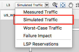Simulation is visible in the network plot by selecting the Simulated Traffic view of the Network Plot drop-down in the left side of the visualization toolbar. In the simulated traffic view, the interface utilization is determined by the sum of all demand traffic routed through each interface divided by the associated circuit capacity. The network plot illustrates the utilization of each interface by the color and amount each interface is filled. More in-depth measured information and simulated results are available in the Property Tables.

Example: Simulation of an Interface Failure

In WAE Design do the following tasks:

1. Open us_wan_L1.txt and make sure you have the network plot set to the Simulated Traffic view as shown above.
2. Right-click on the interface from site SJC to site KCY and select Filter to Demands through selected interface -> All
3. Note the Demands Property Table now has 5 of the 95 demands selected. Select a Demand from er1.sjc to er1.wdc to see the simulated path of the demand on the network plot.
4. Right-click on the circuit between site SJC and site KCY and select Fail.
5. Observe the dashed line which represents the new simulated path the demand would take.
6. Click an empty area of the plot to de-select the demand and also observe the impact on the overall topology of that circuit failure. Note that this failure caused traffic demands to shift, resulting in congestion between site WDC and site NYC.
7. When finished right-click an open area of the plot and select Recover.

Example: Simulation of an IGP Metric Change

In WAE Design do the following tasks:

1. Open 2 copies of the model us_wan_L1.txt
2. Make sure you have the network plot set to the Simulated Traffic view as shown above.
3. On one of the copies, right-click on the interface from site SJC to site KCY and select Properties
4. Change the metric on the interface on cr1.sjc to cr1.kcy from 74 to 70 and select OK.
5. Toggle between the plan files to observe the difference before and after.
6. To run a report of the differences, select Tools -> Reports -> Compare Plans
7. Run a report to compare the demand routings between the plans and observe the results of the report. Note the various fields such as path metric and simulated latency differences before and after.

Example: Simulate Adding a New Customer to the Network

In WAE Design do the following tasks:

1. Open the model us_wan_L1.txt
2. Make sure you have the network plot set to the Simulated Traffic view as shown above.
3. Select Insert -> Demands -> Demand
4. In the Demand Properties menu, set the following fields
   • Name: New_customer
   • Source: er1.bos
   • Destination: er1.mia
   • Traffic: 700 (mbps)
   • Select OK.
5. View the impact of the demand on the topology.
6. Find the demand in the Demands table, right-click and select Plot Demand.

A brief deep-dive on WAE simulation:

If you browse the WAE Design RPC API documentation on DevNet, you will notice there are two aspects to a simulation.

1. The route simulation will route the LSPs and demands based on the network state, discovered LSP paths and metrics and simulate the paths if not available. From the route simulation, you can determine the paths of the LSPs and demands through the network.

2. The traffic simulation will determine the utilizations based on the route simulation.

The Simulation Analysis Tool

In the previous section, you simulated the failure of a circuit and observed the impact. You can simulate failures of other objects as well. However, if you want to find out which failure will cause the greatest impact to the topology, rather than simulate each failure one by one you can use the Simulation Analysis.

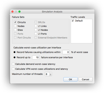
1. Select Tools -> Simulation Analysis
2. Select the objects to examine and click OK

The Simulation Analysis tool will go through each object in the selected properties table, simulate the failure and record the impact. An example of this is shown for circuits in the animated picture below.

When the Simulation Analysis tool completes, you will now be able to see the Worst-Case and Failure Impact traffic views. The Worst-Case traffic view essentially says some failure somewhere will cause traffic to shift and this link will reach the utilization level. To see the object that caused this utilization level, right-click on an interface and select “Fail to WC”. This will take you to the Simulated Traffic view with the failure applied. In contrast, the Failure Impact view displays the objects according to the impact they will have on the topology if they fail.

Conclusion

Using the WAE Design application, you can simulate a variety of “what if” scenarios. Some examples include simulating changes in topology, traffic or configured properties such as metrics. Simulation is a fundamental aspect of WAE and the capabilities of the WAE Design application are also available via API, future releases will use the API for automated workflows. Additional simulation and analysis tools are also available via WAE function packs.

Please check out our other tutorials to explore additional features and capabilities of WAE.

WAE Design Quick Start Guide.