
Network Predictive Analysis: A Journey into Traffic Forecasting with Deep Learning
Context
This development complements the features of Cisco WAN Automation Engine (WAE). WAE is a software tool that permits definition, maintenance and monitoring of a network. It can gather and use information coming from snapshots of the topology, device configurations and telemetry from an operational network. The approach presented here makes use of SNMP traffic data collected by WAE, to which a model has been fitted. Currently, the model is built based solely on traffic information. However, ideally, the project could mature into one that is suitable for production, where additional telemetry-based features of the network are brought in, e.g., number of paths and link failures. The model can be used as an estimator for what if scenarios, predicting a change in the traffic and thus anticipating the need or ability for a network change. A first application could be the provision of future network maintenance windows. Knowing in advance the suitable time and values of the traffic would allow for an optimised maintenance process, opening the window for anticipated network adjustment.
Introduction
With the development of programmatic network APIs and model-driven architectures, network operations are more and more automated. Being able to predict network state in the future allows for the orchestration and path computation engines to figure out network issues before they impact operational performance, to estimate best and feasible network or infrastructure maintenance windows, to plan for optimum capacity upgrade or traffic engineering re-optimisation as well as provide resource allocation with guaranteed service level agreement. Amongst all the key performance indicators available our project aims to forecast the per-interface traffic utilisation variable to address the specific challenge of finding the best maintenance window. When traffic is predicted on all the network interfaces, Cisco WAE algorithm for demand deduction can be used to build the related predicted demands i.e. forecasted traffic matrix from source to destination. When traffic matrix for demands is available, Cisco WAE impact analysis capability allows to compute what if analysis and provide with the state of the network in case of link or node failure. Then, it is possible to get the list of all the feasible maintenance windows not violating any specified maximum link utilisation thresholds and schedule for the less impactful. The main hypothesis to our predictive analysis project is that the network traffic utilisation can be collected as a multiple variables time series where each variable represents per-interface traffic utilisation in a specific direction over time. From experience, we can also make the hypothesis that the time series will exhibit seasonality and trend.
Data
The dataset comes as a collection of plan files. The collection spreads across 3 months with acquisitions made every 10 minutes. Each plan file represents a snapshot of the network state at a given point in time. Although its content describes various components of the network, this project focuses on the Traffic Measurements of the Interfaces. Additionally, a second dataset is used. It is a 1-day dataset with a 15-minute cadence and information on Demand Traffic. This is used for comparing the performance of the proposed approaches. Finally, the sequence of plan files is interpreted as a time series.
Dataset of the Interface Traffic
The training is done on the Traffic Measurement of an interface, with unique keys Node-Interface (Fig.1, Fig. 2). The model definition is based on data for a single interface.
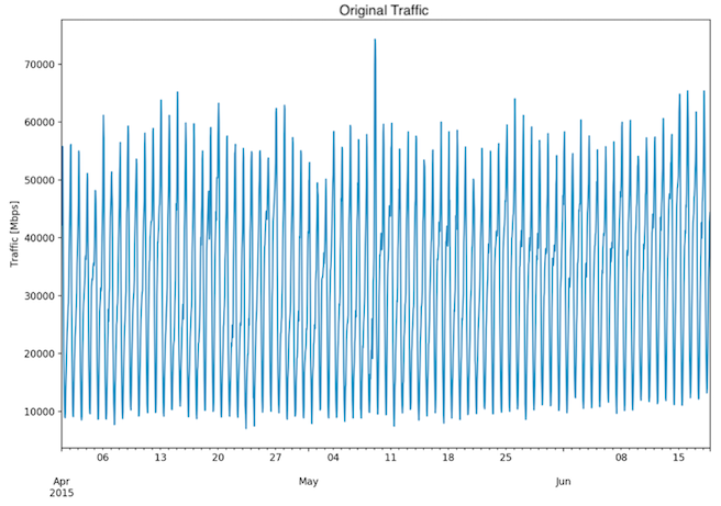
Fig. 1: Three month dataset - Original traffic
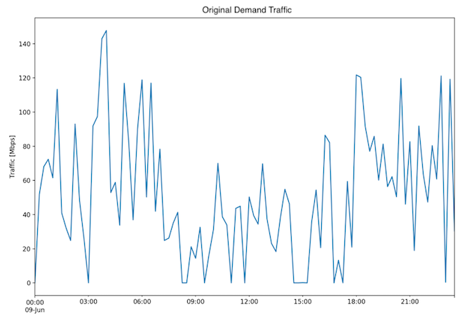
Fig. 2: One day dataset - Original traffic
Exploratory Data Analysis
The quantitative data has been explored through graphical and numerical summaries.
Distribution
The Box Plot (Fig. 3), histogram and density plot (Fig. 4) of the traffic variable show that the 3-month data is skewed to the right. A skewness value of 0.288 was found, with the p-value of 3.54e-05. The distribution shows 3 peaks and is thus multimodal: there are low traffic (< 10 Gbps), medium-low traffic (~ 30 Gbps) and medium traffic (~ 50 Gbps).
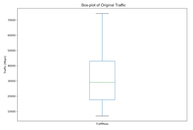
Fig. 3: Three month dataset - Box plot of original data
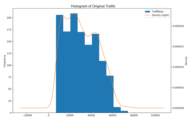
Fig. 4: Three month dataset - Histogram and distribution plot of original data
The 1-day dataset is similarly skewed to the right (Fig. 5, 6), with a single peak, a skewness value of positive 0.855 and a p-value of 0.0059.
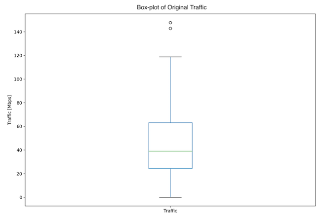
Fig. 5: One day dataset - Box plot of original data
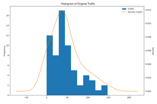
Fig. 6: One day dataset - Histogram and distribution plot of original data
Measures of centrality and variability
In the case of the 3-month dataset, the mean of 30699.8 Mbps and median of 29073.57 Mbps confirm the skewness of the data (Fig. 3, Fig. 4). The standard deviation is 14826.39 Mbps and IQR is 25365 Mbps, with Q1: 17696 Mbps and Q3: 43061 Mbps. This means that the majority of the traffic is between 15873.41 and 45526.19 Mbps. An overview of both datasets is given in the Table 1.
| Measure | 3-month dataset | 1-day dataset |
|---|---|---|
| Count | 1268 | 96 |
| Mean | 30699.80 Mbps | 52.29 Mbps |
| Median | 29073.57 Mbps | 46.78 Mbps |
| Standard deviation | 14826.39 Mbps | 37.51 Mbps |
| Minimum | 7046.44 Mbps | 0.03 Mbps |
| 25% | 17696.04 Mbps | 24.84 Mbps |
| 50% | 29073.57 Mbps | 46.78 Mbps |
| 75% | 43061.07 Mbps | 79.71 Mbps |
| Maximum | 74321.33 Mbps | 147.74 Mbps |
| Variance | 219821840.43 Mbps2 | 1407.00 Mbps2 |
| Range | 67274.89 Mbps | 147.71 Mbps |
| IQR | 25365.03 Mbps | 54.87 Mbps |
Table 1: Measures of centrality and variability
Outliers
There were no outliers in the 3-month data. There were 2 outliers in the 1-day dataset: 142.91, 147.74.
Decomposition
The dataset has been decomposed in seasonality, trend and cycle and residuals. There was no clear proof of a trend but there was proof of a 24-hour seasonality in the case of the 3-month dataset (Fig. 7, Fig. 8).
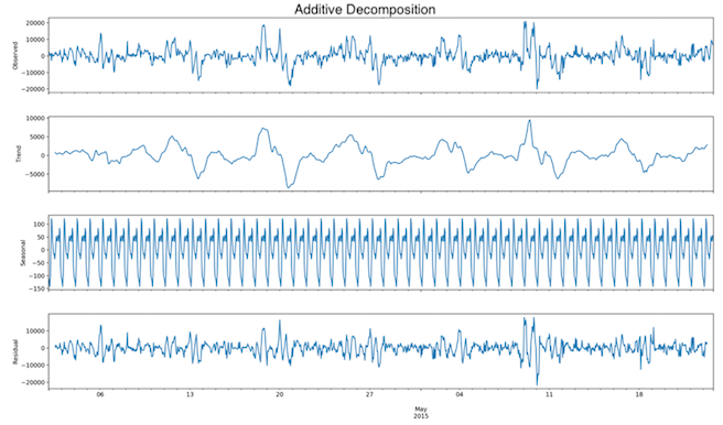
Fig. 7: Three month dataset - Time series decomposition of seasonally differenced data
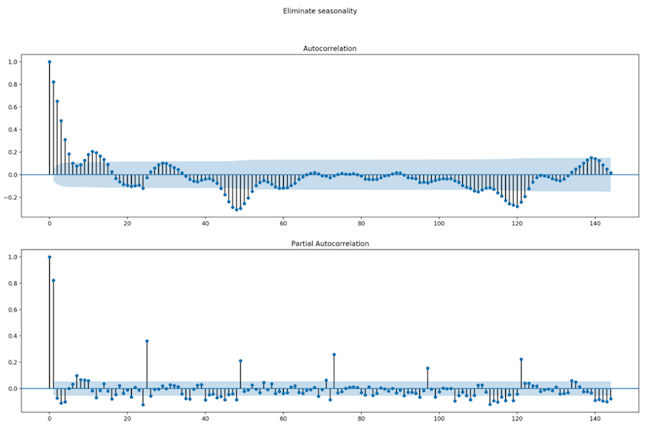
Fig. 8: Three month dataset - ACF and PACF plots of seasonally differenced data
The seasonality for the 1-day dataset was half an hour (Fig. 9, Fig. 10).
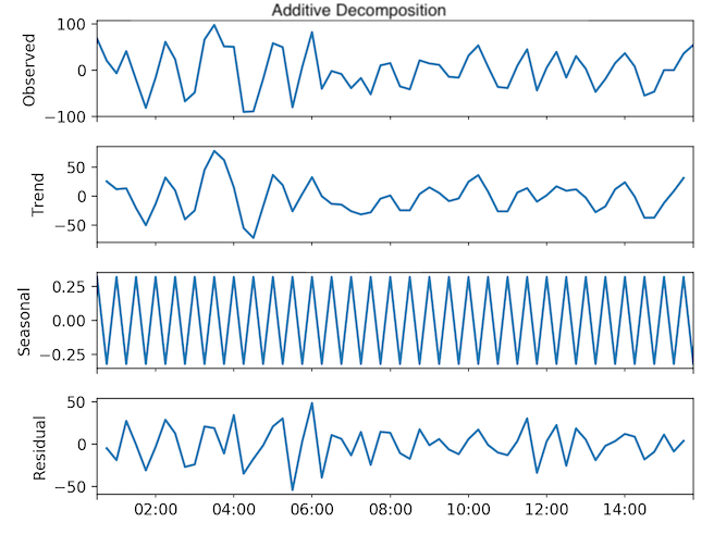
Fig. 9: One day dataset - Time series decomposition of seasonally differenced data
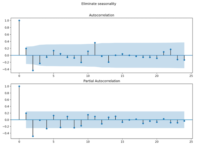
Fig. 10: One day dataset - ACF and PACF plots of seasonally differenced data
Preprocessing
For reasons of content simplification, we present here the preprocessing of the 3-month dataset. The 1-day dataset has been similarly preprocessed.
Data quality, missingness and resampling
The 3-month dataset had missing plan files on several occasions. The missing data has been compensated for. After examination, it has been concluded that there is no pattern in the missing data, that the missing data does not depend on its missing value, and that there is little missingness. Careful analysis revealed that a resampling based on a 1 hour average can not only provide a good estimate of the original dataset, but also decrease the computation time. Therefore, the data has been resampled.
Skewness
Although the measures of central tendency, mean and median are close to one another, the positive skewness value 0.288 shows that the dataset is still skewed to the right. The p-value for the null hypothesis that the data follows a Normal distribution is small, meaning that there is a low chance. Therefore, the data is corrected for skewness with Box-Cox transformation such that the dataset comes closer to a Normal distribution.
Standardisation
Furthermore, the data is standardised with the Min-Max. Once the transformations have been applied, the skewness is -0.0052 and the p-value is 0.939, meaning that there is a 93% chance that the data follows a Normal distribution (Fig. 11).
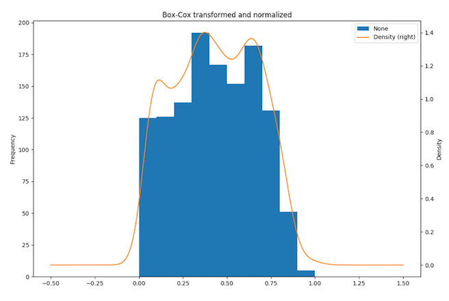
Fig. 11: Three month dataset - Histogram and distribution plot of transformed data
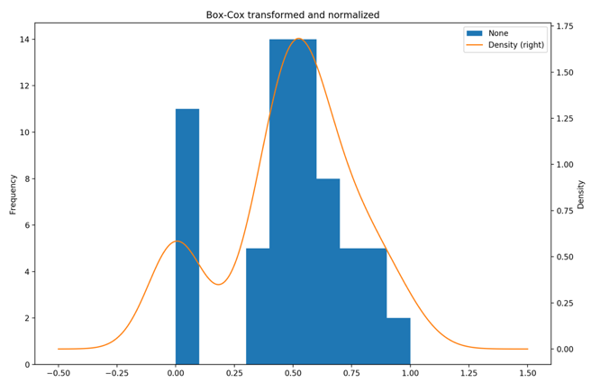
Fig. 12: One day dataset - Histogram and distribution plot of transformed data
Stationarity
The augmented Dickey-Fuller test has been used for assessing the stationarity. The H0 hypothesis: data is non-stationary, is confirmed by the Test-statistic being greater than the 1% critical value. Table 2 shows the stationarity values. After separating the seasonality from the data by means of differencing, the p-value stays below 0.05 and the Test-statistic drops lower than the 1% critical value -3.43. Thus, one can reject the null hypothesis and accept the alternative hypothesis that the data is stationary.
| Measure | Results of Dickey-Fuller Test: Original dataset | Results of Dickey-Fuller Test: Transformed dataset |
|---|---|---|
| Test Statistic | -2.980236 | -2.870370 |
| p-value | 0.036782 | 0.048904 |
| # Lags Used | 23 | 23 |
| # Observations Used | 1244 | 1244 |
| Critical Value (5%) | -2.863866 | -2.863866 |
| Critical Value (1%) | -3.435618 | -3.435618 |
| Critical Value (10%) | -2.568008 | -2.568008 |
Table 2: 3-month Dataset - Dickey-Fuller Test for stationarity
Postprocessing
The predictions are made on transformed data. A back-transformation of Min-Max standardisation and Box-Cox is applied before giving the final traffic prediction.
Modelling
Pipeline
The development process is illustrated in Fig. 13.
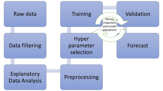
Fig. 13: Development pipeline
Model
For reasons of content simplification, we present here the methodology applied to the 3-month dataset. The learning phase is similar for the 1-day dataset.
Method
The authors of this project have come to the current solution through an iterative process. Based on our trials, the traditional statistical methodologies, such as simple linear regression and seasonal ARIMA have not had a good performance score on test data. Thus, a more modern approach has been considered: the Long Short-Term Memory Recurrent Neural Networks (LSTM). For training phase, the RNN receives as input the current and seasonally neighbouring traffic values. LSTM then fits a non-linear model to the training data. Next, K-fold cross-validation is used. This splits the dataset in subsets, computes a model for each training subset and measures the scores of the model on unseen validation data. In doing so, cross-validation ensures model definition without overfitting. Finally, a new dataset is brought in, as one would do in production. This dataset is for test purposes and its associated score can be compared to the training one, to understand how biased and how good the model is performing. The output of the LSTM RNN is given as a single traffic value per point in time.
Assumptions
At present, the problem was simplified by assuming that the traffic time series is self-descriptive. I.e., there are no external factors that influence the trend, seasonality, residuals. Currently, the training and predictions are done on a node-interface-level. An enhancement to the tool can be that of introducing other telemetry data as new features (e.g. traffic of other interfaces from the same node, link failures, path counts).
Overview of techniques
The traffic dataset can be considered a time series. A first attempt at estimating the dataset has been performed using simple linear regression. Along the development of this project several other approaches have been evaluated. These methods are autoregressive:
- ARIMA (Autoregressive Integrated Moving Average) with parameters (p=5, d=1, q=2)
Non-seasonal ARIMA proved to perform rather poorly. One of the limitations of ARIMA is that it cannot include information about the seasonality component. Furthermore, although one-step out-of-sample forecasting results were close to ground truth, it becomes unreliable when performing multi-step out-of-sample forecasting.
- seasonal ARIMA with parameters (p=0, d=0, q=1), (P=1, D=1, Q=1, s=24) for the 3-month dataset and (p=1, d=1, q=2), (P=1, D=1, Q=1, s=2) for the 1-day dataset
Seasonal ARIMA has the advantage of separating and describing the time series with its decomposed parts. The original time series showed signs of seasonality, thus, the series has been seasonally adjusted. The 3-month dataset showed strong seasonality within each day, whereas the 1-day dataset showed a seasonality within each half an hour, but with more variability in the length of the seasons. The forecast of seasonal ARIMA was good in the case of the 3-month dataset, where the seasonality could predominantly describe the series; in the case of the 1-day dataset it was less successful.
Deep learning - recurrent neural networks (RNN): Long Short-Term Memory (LSTM) with hyper-parameters: visible layer with 1 input, 1 LSTM hidden layer with 4 neurones, an output layer with a single value prediction, ADAM optimiser and MSE (mean squared error) loss function, batch size 1, and:
- 3-month dataset:
- look back: 24
- epochs: 30
- 1-day dataset:
- look back: 2
- epochs: 100.
- 3-month dataset:
LSTM RNN Motivation
Recurrent neural networks have proven to capture the underlying patterns that describe the time series. The simplest artificial neural network is composed of an input layer and an output layer, and mimics the linear regression. When intermediate layers with hidden nodes are added, the neural network becomes non-linear, as each output of a layer is modified using a non-linear function. As with other datasets, one can extract new features that describe the response. In the case of time series, one can use the lagged values as inputs to the neural network. Such a neural network is called autoregressive. Specifically, the seasonality of the data can be learned by the neural network if the previous data points from the same season are given as input. The traditional neural networks do not have persistence of previous events, i.e., they are not capable of correlating events in a sequence. Recurrent neural networks circumvent this deadlock by introducing loops in the structure of the neural network. These loops allow for information to be passed multiple times through the nodes, essentially learning sequences of information. Basic recurrent neural networks cannot retain context of information by means of correlating data with segments from a long past time point. The constraints of traditional recurrent neural networks are overcome with Long Short-Term Memory RNNs. They are a special case of recurrent neural networks that have a more complex structure with 4 internal layers. Each layer acts as a gate, extracts information and updates the state of a cell based on the information that can be passed further.
Model Training
Description
Patterns in the network traffic data can be learned during the training phase. As a result, a model that captured the features of the data is defined. This can further be used for future predictions.
Method
The LSTM RNN uses traffic time-series and past values from the same season as input for the visible layer. Each such feature has a weight associated with it based on the hidden layer. The RNN’s hyper-parameters are customisable. The model is defined by the weights and at the end of the training phase, the model can be saved in memory.
Assumptions
There is one LSTM RNN model per interface. It is assumed that a model from one interface would not work on a different one. Furthermore, the training does not incorporate external information about the traffic on a specific interface.
Model Forecasting
Description
The offline training phase has provided a model for future use. This LSTM model can ingest a window of traffic data, as past seasonal points, and can make a forecast of the upcoming traffic. If needed, the RNN gives room for improvement. One is able to inject new training data and actualise the model by building on top of the original one, effectively adding to the initial training. This ensures a forecast in the context of past, but also recent or new events.
Method
The offline-built model is loaded and fed with new input data, i.e., the traffic values from the last season. Output values of the RNN will represent forecasted traffic based on the historical data. The predicted data provides a basis for scheduling the maintenance of the network. Moreover, the traffic can be fed back in order to estimate demands of the network and understand whether a certain threshold will potentially be exceeded.
Results
Both datasets had good forecasting, LSTM RNN outperforming traditional and seasonal ARIMA.
Three-month dataset: Interface Traffic
The RMSE for the 3-month dataset was 2608.65 Mbps, a value very low considering that the range of the data is 67274.89 Mbps and that the standard deviation is 14826.39 Mbps. Figures 14, 15, and 16 show the forecasts.
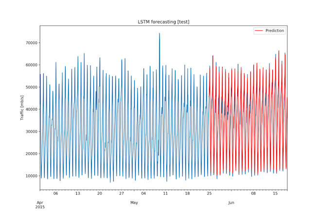
Fig. 14: Three month dataset - Forecast on test set (1/3)
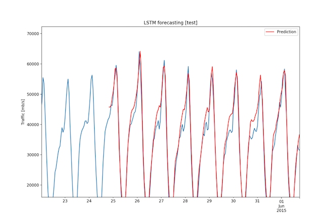
Fig. 15: Three month dataset - Forecast on test set (2/3)
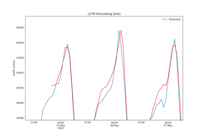
Fig. 16: Three month dataset - Forecast on test set (3/3)
One-day dataset: Demand Traffic
The RMSE was 43.56 Mbps, a value rather high considering that the range of the data is 147.71 Mbps and that the standard deviation is 37.51 Mbps. Nevertheless, as it can be seen in the Figure 17, the predictions follow the pattern of the ground truth. One could consider improving the model by extending the neural network, bringing in more training data or adjusting the hyper-parameters of the RNN.
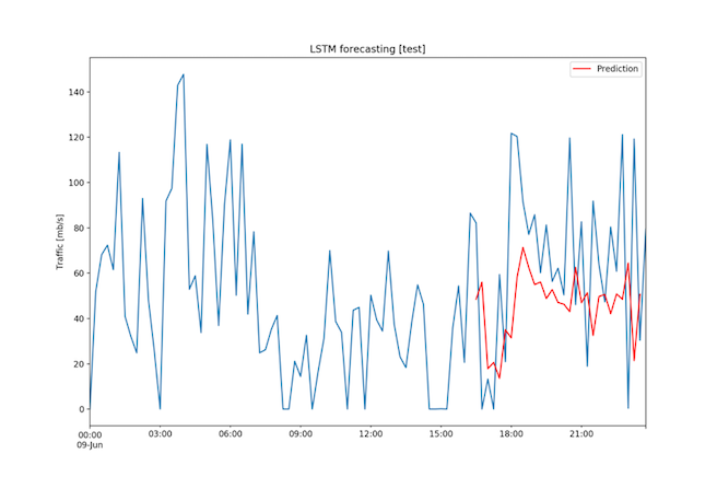
Fig. 17: One day dataset - Forecast on test set
Evaluation
Model Validation
Description
The data has been segmented in two parts: training and test. The training data represented 67% of the original data. Model performance has been assessed using the loss function mean squared error on all three parts of the dataset: training, validation, and test.
Method
K-fold cross-validation with K=10 was used for subsampling the training dataset and computing the fitness measure for the K models. The best model had an MSE error of 0.0016 for the 3-month dataset and an MSE error of 0.0583 for the 1-day dataset. The training scores are shown in original scale in Table 3.
| Measure | 3-month dataset | 1-day dataset |
|---|---|---|
| MSE | 7461821.55 Mbps2 | 1153.38 Mbps2 |
| RMSE | 2731.63 Mbps | 33.96 Mbps |
Table 3: LSTM Training scores
Model Test
Description
33% of the data was put aside for testing purposes, i.e., no bias had been introduced by using this data in the training phase. The values have been given as input to the RNN and the resulted forecast was compared to the ground truth. The performance of the model on the test data has been assessed using the loss function mean squared error. The test scores are summarised in transformed and original scale in Table 4.
| Measure | 3-month dataset | 1-day dataset |
|---|---|---|
| MSE in transformed scale | 0.00135 | 0.07561 |
| RMSE in transformed scale | 0.03681 | 0.27498 |
| MSE | 6805089.28 Mbps2 | 1898.08 Mbps2 |
| RMSE | 2608.65 Mbps | 43.56 Mbps |
Table 4: LSTM Test scores
The Journey Continues
The work presented here is a piece of the analytics puzzle. In order to take this to the production level, more pieces need to be added:
- decrease computation time
- deployment
- lifecycle management of the pipeline
- scalability
- testing
- recurrent training
The deployment would result in an intelligent platform that can be fed traffic data, learn from it and forecast future time points. The advantage of NNs that learn from new data would increase the robustness and flexibility of the model to a large variety of data and keep up with the latest traffic patterns.
The results aforementioned add to the confidence in network automation. Production environments could intelligently use predictions to anticipate events and thus keep up with the volatility of network demands.
Leave a Comment