
Cable Management with ZTP
Foreword
A while ago I wanted to refresh my knowledge of Python and get familar with JSON data structure. I decided to create a small project to help me verify that all the connections from and to newly inserted devices in my lab were correct and functional. The script in this blog may not be very Pythonesque :) as I was still learning Python but it does the job.
Introduction
Cable Management is a a key element of provisioning a device, after installing the device, inserting the optics and cabling everything, we would like to know if everything has been setup correctly before starting the configuration process. In this blog I will go over the visualization part of the cable management, I will go over the verification process in part 2.
This example replies on LLDP to obtain information from the neighbors, LLDP provides the following usefull information:
- The local/remote interfaces for each connection
- The neighbor chassis identification
- The neighbor device name
- The neighbor device description (PID and SW version if the neighbor is IOS-XR)
- The neighbor management IPv4/IPv6 address (if configured)
Graph
Graph visualization is a way of representing structural information as diagrams of abstract graphs and networks. It has a wide range of application including database, bioinformatics software engineering and networking.
Their are multiple formats use to describe graphs: DOT, GXL, GRAPHML and multiple tools to generate and process graph. In my research, I found Graphviz and Gephi to be the most used. Gephi used the GEXF (Graph Exchange XML Format) language internally and includes a set of tools that can generate and/or process various format, it also can be enhanced using plugins and found out that there is a JSON export plugin.
Edges and Nodes
For network graph, we define a node as a LLDP speaking device and an edge as an LLDP learned connection between 2 nodes. The JSON format exported by Gephi can be interpreted in python as a dictionary of an edges list and a nodes list.
graph = {}
graph['nodes'] = []
graph['edges'] = []
A node or an edge is represented in Python using a dictionary that has some mandatory and some optional keys. I decided to organize all the optional parameters in a dictionary under the optional “attributes” key. The “label” (name) and “id” (sequential number) keys are mandatory for both edges and nodes, for edges the “source” and “target” keys are also mandatory to define the origin and destination node of each edge. Some of the key/value pairs in the “attribute” dictionary are not taken from the “show lldp neighbor” output but from the “show controller interface” output and can vary from platform to platform.
I included the Digital Optical Monitoring (DOM) parameters collected from the “show controller” command. Not all transceivers supports the DOM feature but if supported, it provides a good overview of the quality of the signal received on all the transceiver lanes. It also alow you to monitor the temperature and Vcc reported by the transceiver.
The “attributes” dictionary can be customized to include any command output you may find relevant.
The following JSON dictionay describes an example of a node and edge.
node = {
  "label": "",
  "id": "",
  "attributes": {
     "title": "",
     "chassis id": "",
     "system description": "",
     "mgmt address": {
       "IPv4": "",
       "IPv6": ""
     }
  }
}
edge = {
      "label": "",
      "source": "",
      "target": "",
      "id": "",
      "attributes": {
         "remote interface": "",
         "local interface": "",
         "title": "",
         "operational values": {
            "speed": "",
            "duplex": ""
            },
         "optics": {
            "media type": "",
            "vendor": "",
            "PN": "",
            "waveLength": "",
            "DOM": {
               "temp": "",
               "voltage": "",
               "lane 0": {
                   "Tx power": "",
                   "Rx power": ""
                },
                "lane 1": {
                   "Tx power": "",
                   "Rx power": ""
                 },
                 "lane 2": {
                    "Tx power": "",
                    "Rx power": ""
                 },
                 "lane 3": {
                    "Tx power": "",
                     "Rx power": ""
                 }
            }
         }
      }
   }
Workflow
The python script can be downloaded and executed trough the ZTP process. The script will perform the following tasks:
- Create a configuration file that enable all the relevant interfaces and activate LLDP
- Apply the configuration
- Iterate through the list of LLDP neighbors and creates the nodes and edges list
- Populate the edges with the optics values
- Save the graph on the local disk
- Export the graph via HTTP POST to a web server
Creating the configuration file
This function creates a configuration file based on the list of interfaces that we want to use for neighbors discovery, we can sepcify a type of interface or specific interfaces i.e:
LLDP_INTF = ['TenGigE0/0/0/10', 'FortyGigE', 'HundredGigE']
Once the configuration file is created we apply it to the device using the ztp_helper function “xrapply”.
Creating the graph
We start by discovering all the neighbors using the “show lldp neighbors” and “show lldp neighbors detail” commands, once all the neighbors are discovered, we populate the node dictionary with the values of the following keys:
- Id: A sequential number starting with the device itself (id=1)
- Label: The hostname of the neighbor with the domain name stripped out
- Chassis id: The mac address used to identify the neighbor
- System Description: IOS-XR devices use their PID and SW version
- Management IPv4 address: If present
- Management IPv6 address: If present
Similarly, the edge dictionary is populated with the values for the folowing keys:
- Id: A sequential number
- Source: The source node ID which is always 1 since the graph is rooted with the device itself
- Target: The target node ID
- Label: A 2 lines string with the local interface of the device on top
- local Interface
- Remote Interface
- Title: A 2 lines string with the local interface of the device on top
The remaining key/value pairs in the “attribute” dictionary are not taken from the “show lldp neighbor” output but from the “show controller interface” output and can vary from platform to platform. I included the Digital Optical Monitoring (DOM) parameters collected from the “show controller” command. Not all transceivers supports the DOM feature but if supported, it provides a good overview of the quality of the signal received on all the transceiver lanes. It also allows you to monitor the temperature and voltage reported by the transceiver. Once all the values for the nodes and edges are poulated , we save the JSON file on the local disk.
Exporting the graph
I wanted to export the JSON graph file directly from the device to an apache web server using HTTP POST, Apache supports PUT and POST if you allow these metodods in the configuration of the virtual server but you still need a way to process the request. I create a simple PHP handler for this purpose. The PHP script simply copy the file to a specified directory and use the name provided in the HTTP POST form “file_contents”. It return the status of the operation in JSON format for easier processing by the script.
<?php
$uploaddir = realpath('./datasources') . '/';
$uploadfile = $uploaddir . basename($_FILES['file_contents']['name']);
	if (move_uploaded_file($_FILES['file_contents']['tmp_name'], $uploadfile)) {
		$data = array("status"=>"success","output"=>$_FILES);
        echo json_encode($data);
	} else {
		$data = array("status"=>"error","output"=>$_FILES);
        echo json_encode($data);
	}
	//echo 'Here is some more debugging info:';
	//print_r($_FILES);
?>
IOS-XR comes standard with urllib, urllib2 and httplib which can be used to perform an HTTP POST request. Unfortunatly neither urllib nor httplib directly support mime type “multipart/form-data” and I had to create 2 functions for this purpose.
def post_multipart(self, host, selector, fields, files):
  """
  Post fields and files to an http host as multipart/form-data.
  @param host: the hostname of the server to connect to.  e.g.: www.myserver.com
  @param selector: where to go on the host. e.g.: cgi-bin/upload.php or datasources/upload, etc..
  @param fields: a sequence of (name, value) elements for regular form fields.  For example:
  [("vals", "16,18,19"), ("foo", "bar")]
  @param files: a sequence of (name, file) elements for data to be uploaded as files. For example:
[ ("Erebus", open("/images/me.jpg", "rb")) ]
  @return: the server's response page.
  """
  content_type, body = ztp_script.encode_multipart_formdata(fields, files)
  h = httplib.HTTPConnection(host)
  headers = {
  'User-Agent': 'python_multipart_caller', 'Content-Type': content_type
  }
  h.request('POST', selector, body, headers)
  res = h.getresponse()
  return res.read()

def encode_multipart_formdata(self, fields, files):
  """
  @return: (content_type, body) ready for httplib.HTTP instance
  """

  BOUNDARY = '----------ThIs_Is_tHe_bouNdaRY_$'
  CRLF = '\r\n'
  L = []
  for (key, value) in fields:
    L.append('--' + BOUNDARY)
    L.append('Content-Disposition: form-data; name="%s"' % key)
    L.append('')
    L.append(value)
  for (key, fd) in files:
    file_size = os.fstat(fd.fileno())[stat.ST_SIZE]
    filename = fd.name.split('/')[-1]
    contenttype = 'application/octet-stream'
    L.append('--%s' % BOUNDARY)
    L.append('Content-Disposition: form-data; name="%s"; filename="%s"' % (key, filename))
    L.append('Content-Type: %s' % contenttype)
    fd.seek(0)
    L.append('\r\n' + fd.read())
  L.append('--' + BOUNDARY + '--')
  L.append('')
  body = CRLF.join(L)
  content_type = 'multipart/form-data; boundary=%s' % BOUNDARY
  return content_type, body
Visualizing the graph
To render the graph correctly, we will need the help of some javascript libraries, I found out that vis.js has the capability to import JSON graph created with Gephi and has strong support for network graphs. An example of rendering the JSON graph file is shown below:
var graphJSON = loadJSON("./datasources/lldpNeighbors.json");
var parserOptions = {
  edges: {
    inheritColors: false
  },
  nodes: {
    fixed: true,
    parseColor: false
  }
}
// parse the gephi file to receive an object
// containing nodes and edges in vis format.
var parsed = vis.network.convertGephi(graphJSON, parserOptions);

// provide data in the normal fashion
var data = {
  nodes: parsed.nodes,
  edged: parsed.edges
};
// create a network
var network = new vis.Network(container, data);
I also needed a file browser that supports browsing and selecting server-side files. I found a jQuery plugin at A Beautiful Site that solved that issue. It’s an AJAX file browser with server-side connector scripts for JSP, PHP, ASP, and others. The nice thing about this script is that it returns the selected file path as a string and with a bit of manipulation, I built the webapp’s file tree with the following script:
$(document).ready(function() {
  $('#loadFolderTree').fileTree({
    root: '/var/www/html/lldpNeighbors/datasources/',
    script: './jquery/connectors/jqueryFileTree.php',
    multiFolder: false },
    function(file) {
        jsonFile = file.replace(/^.*[\\\/]/, './datasources/')
        console.log(jsonFile)
        loadJSON(jsonFile, redrawAll, function(err) {console.log('error')});
  });
});
Finally I divided the web page in 3 sections: The representation of the graph and a dump of the node and edge content when selected in the graph. Here is breakdown of the 3 sections:
The graph
The screenschot below show the graph with one node selected, note that the neighbor has LLDP enabled on the bundled interface: 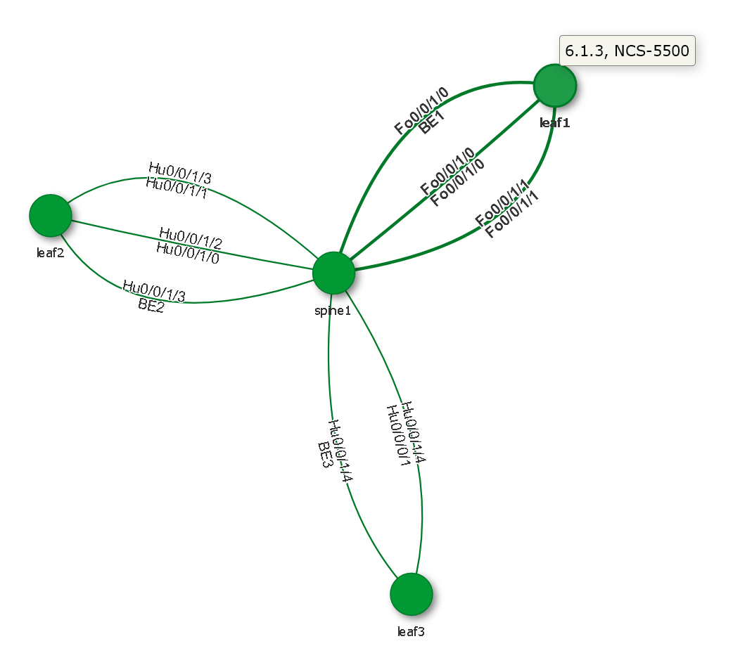
The Node
When a node is selected the node content section is displayed for that node: 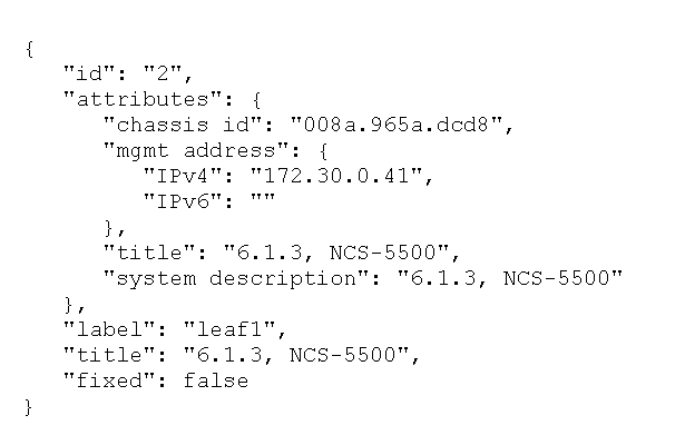
The Edge
When an edge is selected, this section will display the full content of that edge: 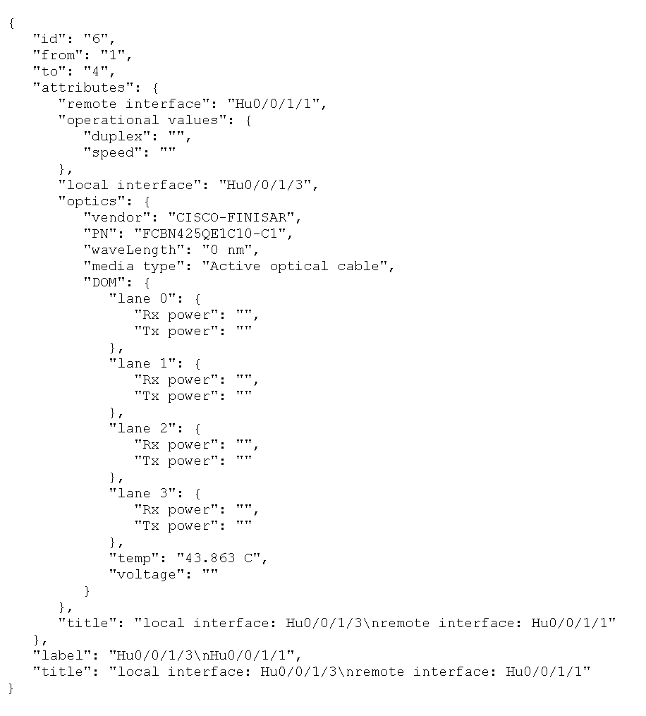
Conclusion
With this example, I was able to go through the process of dynamically creating a data file on the device and export it to an HTTP server. The functions described here can be applied to other scenario where the device being provisioned needs to communicate its topology to a service that will apply specific configuration snipset based on that topology. The complete code is available on github. Feel free to send me your comments.
Leave a Comment